Valuation 101: How to Accurately Determine an Asset’s Worth
Executive Summary
Valuation is the process of estimating the current value of an asset or business by analyzing its future streams of benefits. Under International Financial Reporting Standards (IFRS), fair value is defined as “the price that would be received to sell an asset or paid to transfer a liability in an orderly transaction” (IFRS 13); in essence, it is also the “reasonable price” from the perspective of market participants. From a financial-analysis perspective, valuation aims to assess an asset’s intrinsic value, supplemented by market parameters such as comparable-company valuations, to support decisions involving investment, mergers and acquisitions, financial-reporting disclosure, and financing negotiations. The core principles of valuation include the time value of money, the risk–return relationship—the higher the risk, the higher the return investors require—and market efficiency—if markets are efficient, price is the best estimate of value (Aswath Damodaran, Chapter 6). Common valuation methods include discounted cash flow (DCF), the dividend discount model, the residual income model, relative valuation using multiples, precedent transactions, real options, asset-based valuation, and specialized methods for startups, intangible-asset-intensive companies, crypto assets, real estate, and other special asset classes. This article defines each method, explains its assumptions, formulas, and procedures, and uses tables and diagrams to describe its strengths, weaknesses, required data, and applications. It concludes with a valuation comparison table, a due-diligence checklist, common pitfalls, and practical recommendations.
Definition and Objectives of Valuation
Valuation is the process of estimating the current value of an asset, business, or investment by analyzing future cash flows or earnings while considering market references, risk discounts, and other factors. In academic and professional practice, valuation can be divided into two major approaches: absolute valuation, based on discounting the asset’s own forecast cash flows or earnings, and relative valuation, based on the market-price multiples of comparable assets.
The objectives of valuation include investment analysis and decision-making—determining whether an investment is worthwhile—corporate acquisitions and private equity—determining acquisition value—financial-statement disclosure, such as fair-value measurement, and tax or legal disputes, such as estate-tax or breakup-fee calculations. IFRS 13 states that fair value should reflect the perspective of market participants and should not consider transaction costs (IFRS 13), emphasizing the price in the most advantageous market. Therefore, valuation must consider both an asset’s ability to generate income and prevailing market conditions.
Fundamental Principles of Valuation
-
Time Value of Money: Under the time-value-of-money principle, “one dollar today” is worth more because it can be invested. Discounted cash flow models are built on this foundation, discounting future cash flows back to the present according to their risk. The concept can be summarized as follows: money has the potential to earn an investment return, so receiving it earlier makes it more valuable (Investopedia: Time Value of Money). Mathematically, the present-value formula is:
\[PV = \sum \frac{CF_t}{(1+r)^t}\]where \(r\) is the discount rate (Investopedia: Discounted Cash Flow).
-
Risk/Return Trade-off: Investors must receive higher returns for bearing greater risk. The capital asset pricing model (CAPM) states that an asset’s expected return should be positively related to its systematic risk, or beta. In other words, the greater the risk—the larger the beta—the higher the return investors require (ACCA: The Risk and Return Relationship). Portfolio diversification can eliminate unsystematic risk, leaving only market risk to be compensated (ACCA: The Risk and Return Relationship). Accordingly, valuation usually represents risk through the cost of capital, such as the weighted average cost of capital (WACC) or cost of equity (\(K_e\)), and discounts cash flows to reflect different risk levels.
-
Market Efficiency: If markets are efficient, asset prices already reflect all available information and are unbiased estimates of value (Aswath Damodaran, Chapter 6). In a perfectly efficient market, analysts need only “justify” the reasonableness of the market price. If markets are not fully efficient, analysts must use valuation to identify undervalued or overvalued opportunities (Aswath Damodaran, Chapter 6). In practice, markets differ in their degree of efficiency, and research into information asymmetry or behavioral biases can still inform valuation.
Major Valuation Methods
Discounted Cash Flow (DCF)
Discounted cash flow is an absolute valuation method that estimates a company’s current value by forecasting future free cash flow (FCF) and discounting it using an appropriate discount rate (Investopedia: Discounted Cash Flow). The common steps are as follows:
- Forecast future free cash flow: Analysts calculate annual FCF from operating forecasts, including revenue, operating profit, capital expenditure, and working capital. This can be divided into free cash flow to the firm (FCFF) and free cash flow to equity (FCFE). FCFF is generally after-tax operating profit minus investment and working-capital needs, while FCFE additionally reflects debt repayment, new borrowing, and equity issuance.
- Select the discount rate: WACC is generally used for FCFF, while the cost of equity \(K_e\) is used for FCFE (Investopedia: Discounted Cash Flow). WACC reflects the average cost of debt and equity financing and is generally lower than the cost of equity.
-
Calculate present value and terminal value: Divide each period’s FCF by \((1+r)^t\) and sum the results. For value beyond the explicit forecast period, estimate terminal value using either a perpetual-growth model—the Gordon growth model—or an exit-multiple method, then discount it back to the present. An example formula is:
\[\text{Enterprise Value} = \sum_{t=1}^{N} \frac{FCF_t}{(1+WACC)^t} + \frac{FCF_{N+1}}{(WACC-g)(1+WACC)^N}\]where \(g\) is the perpetual growth rate (Investopedia: Discounted Cash Flow).
-
Summary of the process: First, forecast multi-year cash flows. Next, determine the discount rate, either WACC or \(K_e\). Then, discount each period’s cash flow and sum the results. After that, calculate and discount the terminal value. Finally, combine the values to obtain enterprise value.
flowchart TB A[Forecast Future Cash Flow FCF] --> B[Determine Discount Rate WACC or Ke] A --> D[Calculate Perpetual-Growth Terminal Value] B --> C[Calculate Present Value of Each Cash Flow] C --> F[Enterprise Value = Sum of Cash-Flow PVs + Terminal-Value PV] D --> E[Calculate Present Value of Terminal Value] E --> F - Strengths: Strong theoretical foundation and close alignment with fundamentals; can reflect a company’s long-term value; allows detailed modeling using internal financial-statement data.
- Weaknesses: Highly dependent on assumptions such as growth and discount rates, so small changes can produce materially different results; less suitable for startups or stable-growth companies with unstable cash flows; requires extensive financial forecasting.
- Data requirements and adjustments: Requires multi-year financial forecasts, including revenue, expenses, and capital expenditure, as well as a reasonable source for the discount rate, such as CAPM for estimating the cost of equity. Non-operating items, including financial assets, real estate, and corporate debt, require adjustment. Changes in capital structure, large one-time items, and inflation also require special treatment.
- Applicable situations: Most commonly used for stable, mature businesses, such as traditional manufacturing and industries with stable cash flows; subsidiary valuation; greenfield project-investment evaluation; and merger-negotiation scenarios.
Dividend Discount Model (DDM)
The dividend discount model is an intrinsic-valuation method that assumes the company distributes cash to shareholders only through dividends. Its central assumption is that a company’s value equals the present value of all future dividends (Wall Street Prep: Dividend Discount Model). The common Gordon growth model is:
\[P_0 = \frac{D_1}{k_e-g}\]where \(P_0\) is intrinsic value per share, \(D_1\) is the expected dividend in the next period, \(k_e\) is the shareholders’ required rate of return, and \(g\) is the perpetual dividend-growth rate (Wall Street Prep: Dividend Discount Model). Two-stage or multi-stage models calculate and discount dividends separately across different growth stages.
- Strengths: Simple formula focused on shareholder cash flows; suitable for companies with stable dividends and predictable growth.
- Weaknesses: Suitable only for stable dividend-paying companies and ineffective for non-dividend-paying or high-growth companies. If dividend policy is unstable or the growth rate is difficult to estimate, the model becomes unreliable (Wall Street Prep: Dividend Discount Model). It can also undervalue companies that reinvest heavily and pay low dividends.
- Data requirements and adjustments: Requires historical dividend records and a reasonable growth-rate estimate. If dividends are not permanent, a multi-stage model can be used. Treasury shares, special dividends, and other nonrecurring items must be considered.
- Typical applications: Mature blue-chip companies and banks often use this method. When cash flow reaching shareholders cannot be directly observed, dividends serve as a substitute measure.
Residual Income Model
The residual income model values equity by adding the present value of expected economic excess earnings to current shareholders’ equity book value. Its core concept is:
Residual income = Net income − Shareholders’ equity × Cost-of-capital rate (Investopedia: Residual Income Model).
In other words, the company deducts the required equity charge from accounting profit to determine how much “true profit” remains. The general valuation formula is:
\[V_0 = BV_0 + \sum_{t=1}^{N} \frac{RI_t}{(1+k_e)^t}\]where \(BV_0\) is current shareholders’ equity book value, \(RI_t\) is residual income in year \(t\), and \(k_e\) is the cost of equity (Investopedia: Residual Income Model). This resembles the dividend model but uses future earnings after deducting the cost of equity.
- Strengths: Applicable to non-dividend-paying companies or companies with negative cash flow, as long as accounting earnings exist. Required data are usually available from financial statements, and the model highlights the difference between economic and accounting profitability (Investopedia: Residual Income Model).
- Weaknesses: Heavily dependent on estimates of earnings and the cost of capital (Investopedia: Residual Income Model). Financial-statement manipulation or changes in accounting policies can distort residual-income estimates. It is less suitable for high-technology companies whose earnings cannot be forecast reliably.
- Data requirements and adjustments: Requires accurate book equity, with market-value adjustments where appropriate; forecasts of future net income and cost of capital; and removal of nonrecurring gains, losses, and accounting manipulation.
- Typical applications: Suitable for mature businesses and capital-intensive companies such as banks and insurers. It is especially useful when cash flow is unavailable but earnings are predictable.
Relative Valuation: Multiples Such as P/E, EV/EBITDA, and EV/Sales
Relative valuation is market-oriented. It estimates a target’s value by comparing market multiples from peer companies or comparable transactions. Common multiples include price-to-earnings (P/E)—share price divided by earnings per share—enterprise value to earnings before interest, taxes, depreciation, and amortization (EV/EBITDA), and enterprise value to revenue (EV/Sales).
- Calculation method: First select a group of comparable companies similar to the target in industry, scale, growth, and other characteristics. Collect their market values and financial indicators, calculate average or median multiples, and apply the selected multiple to the target company’s corresponding metric. For example, if the peer-group average P/E is 10 times and the target’s earnings per share are 5 currency units, the estimated share price is approximately 50. For EV/EBITDA, calculate the target’s EBITDA and multiply it by the selected multiple to obtain enterprise value.
- Strengths: Simple and intuitive; reflects current market pricing; uses readily available data such as share prices and financial statements; useful as a cross-check for other valuation methods.
- Weaknesses: Ignores company-specific differences. Differences in growth, margins, leverage, and other factors can justify different multiples. Multiples can deviate from fundamentals because of market sentiment, and poor comparable-company selection can distort the valuation. P/E is susceptible to accounting manipulation and applies only to profitable companies (Investopedia: EV/EBITDA or P/E). EV/EBITDA removes differences arising from debt costs, taxes, depreciation, and amortization and can therefore provide a broader measure (Investopedia: EV/EBITDA or P/E), but it excludes capital expenditure (Investopedia: EV/EBITDA or P/E). EV/Sales can be used for high-growth or temporarily loss-making companies.
- Data requirements and adjustments: Requires a peer group and its share prices, market capitalizations, and financial-statement data. Before calculating multiples, analysts usually adjust unusual items, such as one-time income and treasury-share effects. Industry boundaries must be selected carefully.
- Typical applications: Peer-company valuation, public-market pricing, and rapid value estimation. It is often used alongside DCF and precedent transactions to confirm a reasonable range.
Precedent Transactions
Precedent transactions are another form of relative valuation, but the reference points are historical merger-and-acquisition transactions. The basic approach is to identify completed acquisitions involving companies similar to the target in nature and industry, calculate ratios between transaction value and the acquired companies’ financial metrics—such as EV/EBITDA or EV/Revenue—and apply the resulting multiple range to the target company’s corresponding metrics (Corporate Finance Institute: Precedent Transaction Analysis).
- Strengths: Reflects prices that actual buyers were willing to pay and usually includes a control premium. It is particularly important for valuing private companies and acquisitions in specialized industries (Corporate Finance Institute: Precedent Transaction Analysis).
- Weaknesses: The number of comparable transactions is often limited, and much of the information is private or available only through paid databases. Historical transaction multiples may become obsolete under different market conditions. Because transactions involve control, their valuation multiples are often higher than those for minority-equity trading (Corporate Finance Institute: Precedent Transaction Analysis). Buyer type—financial or strategic—also affects the multiple.
- Data requirements and adjustments: Requires collecting and screening relevant M&A transactions by industry, scale, timing, and other criteria, and excluding transactions that do not match the target (Corporate Finance Institute: Precedent Transaction Analysis). Common metrics include EV/EBITDA and EV/Revenue (Corporate Finance Institute: Precedent Transaction Analysis). Where possible, adjust for differences in transaction timing and market conditions.
- Typical applications: Private-company valuation and M&A pricing; can provide an indication of the upper end of market value. It is often presented together with comparable-company valuation in a football field chart (Corporate Finance Institute: Precedent Transaction Analysis).
Real Options
Real-options valuation treats managerial flexibility in investment decisions as an option and assigns value to it. It is commonly applied to projects involving high uncertainty and meaningful strategic choices, such as research and development, capacity investment, and natural-resource development. Real options include the ability to delay investment, expand project scale, temporarily suspend operations, or abandon a plan. These resemble financial-market options but are embedded in business operations (Investopedia: Real Options).
- Pricing logic: Treat the project’s net present value as the underlying asset value, the investment cost as the strike price, and volatility as a measure of risk. The option can be valued using the Black–Scholes formula or a binomial-tree model (Investopedia: Real Options). For example, a new project may be delayed when interest rates are high, similar to holding a European call option.
- Strengths: When uncertainty is high and strategic flexibility exists, this approach captures value ignored by traditional DCF and reflects management’s ability to adjust as markets change.
- Weaknesses: Complex to implement; requires assumptions for volatility, option life, and other parameters that are difficult to observe because there is no traded market price. Results are highly sensitive to parameters and difficult to validate. Analysts need knowledge of financial derivatives or risk making calculation errors.
- Typical applications: Oil and gas, mining, pharmaceutical R&D, and new-technology projects in the technology industry. These areas often involve decisions about timing, expansion, contraction, and abandonment.
Asset-Based Valuation
Asset-based valuation treats a company as a collection of assets and measures total value using book value or replacement value. Common methods include book value and liquidation value. Book value equals total assets minus total liabilities and corresponds to shareholders’ equity reported in the financial statements (Kotak Neo: Asset-Based Valuation). Liquidation value estimates the net value available after assets are sold at market prices during liquidation.
- Strengths: Suitable for asset-heavy companies, unstable cash-flow businesses, or liquidation scenarios, such as real-estate companies, mining, and shipbuilding (Kotak Neo: Asset-Based Valuation). It can provide a lower bound for company value—an asset floor. The approach is transparent whenever the assets can be valued.
- Weaknesses: Ignores future earning power and cannot reflect intangible assets or future growth. Book values may differ substantially from actual market values, for example because equipment has aged or real estate has appreciated, requiring replacement-cost adjustments. For a going concern, asset valuation often understates total value (Kotak Neo: Asset-Based Valuation).
- Data requirements and adjustments: Requires detailed balance-sheet items, including property, plant and equipment, inventory, investments, and real estate, plus fair-value adjustments. Liquidation value must reflect sale discounts and contract-termination costs. All liabilities must be fully included, or future liabilities discounted where appropriate.
- Typical applications: Liquidation valuation, corporate restructuring, and bankruptcy; financial-asset management and special-asset investments such as REITs; and companies whose value is primarily based on production facilities or land.
Valuation of Nontraditional Assets
-
Startups: Because startups lack stable cash flow and mature financial data, specialized methods are commonly used. One example is the venture capital method. First forecast the company’s enterprise value at a future exit date, using comparable-company multiples or financial targets, then discount that amount at a high rate reflecting the investor’s required return, often 20%–50%, to obtain the current pre-money valuation. The calculation must consider post-money valuation and the proportion represented by the investment. For example, assume a startup is expected to be sold for USD 80 million in five years and the investor requires a 30% annual return. Present value is approximately \(80M/(1.3^5) \approx 21.5M\). If the round requires USD 5 million, post-money valuation is approximately USD 26.5 million and the investor owns approximately 19% (Investopedia: Valuing Startup Ventures). Other methods include stage-based valuation and risk-factor methods. Startup valuations are highly unstable and closely linked to product progress, market conditions, and investor expectations.
-
Intangible-asset-intensive companies: These include businesses whose main sources of value are brands or patents, such as software, gaming, and pharmaceutical R&D companies. Applicable methods include the income approach, such as the relief-from-royalty method for brands, which estimates the licensing fees that would have to be paid to use the trademark and discounts them to present value; the market approach, based on similar intellectual-property transactions; and the cost approach, based on replacement cost (Investopedia: Intangible Assets). Projects with R&D flexibility may combine real-options valuation to estimate the growth potential of patents or technology (Investopedia: Real Options). These companies are often difficult to value using ordinary multiples because their profit models and asset structures differ.
-
Crypto assets: Most cryptocurrencies and tokens currently do not generate cash flow, so they cannot be directly valued using DCF or dividend models. Common approaches use on-chain transaction volume or user counts, such as the network value to transactions ratio, compare market capitalization with potential economic value, including through Metcalfe’s law, or treat certain industry tokens as commodities and apply supply-and-demand models. No mature standard currently exists, valuations are highly unstable, and analysis generally depends on relative valuation—such as market-capitalization multiples among tokens in the same sector—and market sentiment.
-
Real estate: The main method is the income approach, which values property using rent or net operating income (NOI) through DCF or capitalization. Common methods include direct capitalization, where value equals NOI divided by the capitalization rate, and discounted cash flow, which forecasts future rental cash flows and adds terminal value. Capitalization rates are usually inferred from market transactions (Altus Group: Discounted Cash Flow in Real Estate). The income approach considers the entire holding period and subsequent sale value and is more comprehensive than a comparison based only on a single point in time (Altus Group: Discounted Cash Flow in Real Estate). Other real-estate methods include the sales-comparison approach, based on recent transactions involving comparable properties, and the cost approach, based on replacement cost.
Examples: Numerical Calculation Demonstrations
Example 1: DCF Valuation of a Listed Company
Assume a mature company has current-year free cash flow of 100 currency units. Cash flow is forecast to grow by 5% annually over a five-year forecast period. WACC is 8%, and the perpetual growth rate is 2%.
| Year | Free Cash Flow (FCF) | Discount Factor (8%) | Present Value (NPV) |
|---|---|---|---|
| 1 | 100.00 | \(1/(1.08)^1 = 0.926\) | 92.59 |
| 2 | 105.00 | \(1/(1.08)^2 = 0.857\) | 90.02 |
| 3 | 110.25 | \(1/(1.08)^3 = 0.794\) | 87.58 |
| 4 | 115.76 | \(1/(1.08)^4 = 0.735\) | 85.06 |
| 5 | 121.55 | \(1/(1.08)^5 = 0.681\) | 82.74 |
| Subtotal: Present Value of Cash Flows | — | — | 438.0 |
| Perpetual Terminal Value, beginning in Year 6 | 123.98, estimated Year 6 FCF | \(WACC-g=6\%\) | 1,388 after calculating perpetual terminal value and discounting to Year 0 |
| Enterprise Value (EV) | — | — | approximately 1,844 |
Detailed calculation: First, discount and sum each year’s FCF to obtain approximately 438. Then calculate the perpetual value at the end of Year 5:
\[TV = \frac{FCF_6}{0.08-0.02} = \frac{123.98}{0.06} \approx 2,066\]Discounting it back to the present gives approximately 1,407. Adding the two produces enterprise value of approximately 1,845. If debt exists, subtracting debt produces equity value. Based on the parameters above, the calculated result is: enterprise present value = 2,245, including discounted terminal value of 1,388 plus discounted FCF of 438.
The following figure shows the sensitivity of valuation to changes in each assumption—an example tornado diagram:
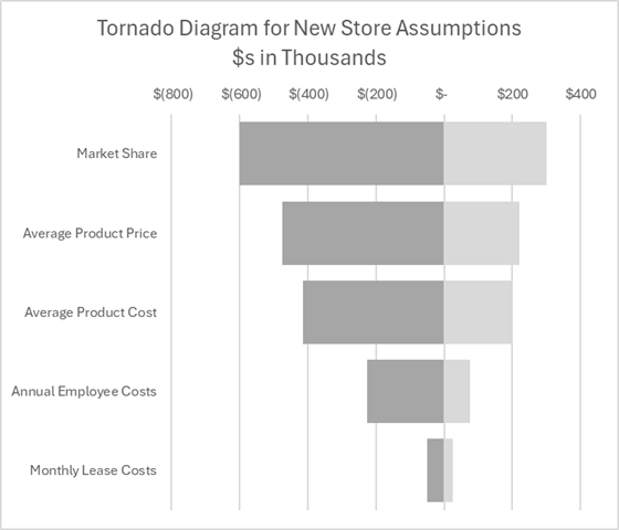
Figure: Example tornado diagram. Each bar represents how a change in one parameter affects enterprise value—the DCF model’s NPV—while other variables remain constant. The discount rate has the largest effect, followed by the growth rate. (CFO Perspective: Tornado Diagrams)
Example 2: Startup Valuation Using the VC Method
Assume a startup is expected to be sold at an exit value of USD 80 million in five years. The venture-capital investor requires a 30% annualized return, or IRR. Calculate the pre-money valuation as follows:
- Estimated terminal enterprise value: USD 80 million
- Discount rate: 30%; five-year compound factor: \(1.3^5 \approx 3.71\)
- Discounted enterprise value: \(\$80M/3.71 \approx \$21.5M\), described here as the current post-money value
- If the financing round requires USD 5 million, post-money valuation = USD 26.5 million, pre-money valuation = USD 26.5 million − USD 5 million = USD 21.5 million, and the investor owns approximately 19%, calculated as \(5/26.5\)
| Parameter | Value |
|---|---|
| Estimated exit value, enterprise value after five years | USD 80M |
| Target annual return | 30% |
| Discount factor, \(1.30^5\) | approximately 3.71 |
| Discounted enterprise value | USD 21.5M |
| Financing amount | USD 5.0M |
| Post-money valuation | USD 26.5M |
| Investor ownership | \(5.0/26.5 \approx 19\%\) |
Example 3: Real-Estate Income Valuation Using DCF
Assume a property has beginning annual net operating income of 1,000, measured in thousands of U.S. dollars. Annual income grows by 2%, and both the discount rate and capitalization rate are 8%. Use a five-year forecast period and capitalize Year 6 NOI to determine terminal value.
| Year | Forecast NOI | Discount Factor (8%) | Present Value of NOI |
|---|---|---|---|
| 1 | 1,000 | 0.926 | 926.0 |
| 2 | 1,020 | 0.857 | 875.1 |
| 3 | 1,040 | 0.794 | 825.9 |
| 4 | 1,061 | 0.735 | 780.2 |
| 5 | 1,082 | 0.681 | 736.6 |
| Subtotal: Present Value of NOI | — | — | 4,143.8 |
| Year 6 NOI, \(1,082 \times 1.02 = 1,104.1\) | — | — | — |
| Terminal Value (TV) | 13,801, calculated as \(1,104.1/8\%\) | Discounted at 0.681 | 9,388.6 |
| Property Value (PV) | — | — | approximately 13,532 |
In addition, the direct-capitalization method simplifies the calculation. Dividing first-year NOI by the capitalization rate gives:
\[\text{Value} \approx \frac{1,000}{0.08} = \$12,500\]This is slightly lower than the DCF result of 13,532 because DCF incorporates future income growth.
Method Comparison Table
The following table summarizes the applicability of different valuation methods to various asset types:
| Method / Asset Type | Listed Company | Private Company / Private Equity | Startup | Intangible-Asset-Intensive | Crypto Asset | Real Estate |
|---|---|---|---|---|---|---|
| DCF, Free Cash Flow | ✔️ | ✔️ | Weak | ✔️, if cash flow can be estimated | ✖️ | ✔️, for income streams |
| DDM, Dividend Discount | ✔️, with stable dividends | ✖️ if no dividends | ✖️ | ✖️ | ✖️ | ✖️ |
| Residual Income Model | ✔️ | ✔️ | ✔️, if profitable | ✖️ | ✖️ | ✔️/✖️, if earnings can be estimated |
| Comparable-Company Multiples | ✔️ | ✔️ | Low reliability | Depends on comparables | Estimate | Limited use, such as REIT multiples |
| Precedent-Transaction Multiples | ✔️ | ✔️ | Low reliability | Depends on transactions | ✖️ | Limited use, requiring comparable transactions |
| Real Options | Weak | Weak | ✔️, where flexibility matters | ✔️, for technology options | ✖️ | Weak |
| Asset-Based | ✖️/Limited | ✔️/Liquidation | ✖️ | Partially applicable, such as IP replacement | ✖️ | ✔️, for land and equipment |
Due-Diligence Checklist and Common Pitfalls
- Validate financial data: Ensure that financial statements are authentic and reliable. Check for manipulation and accounting adjustments, including one-time items, treasury shares, and nonrecurring gains or losses. For private companies, obtain audited statements or tax filings where possible.
- Assess the reasonableness of assumptions: Review forecast growth rates, sources of discount rates—such as CAPM for estimating the cost of equity—and the reasonableness of terminal-growth assumptions. Perform sensitivity analysis on key variables, as illustrated in the example figure, to understand the range of uncertainty.
- Use appropriate market references: Comparable companies and transactions should be similar in industry, geography, and scale. Consider changes in market conditions, including economic cycles, bubbles, and crises.
- Cross-check multiple methods: Combine internal and external valuation results. For example, compare the valuation ranges produced by DCF, trading multiples, and precedent transactions in a football field chart to avoid reliance on a single model.
- Report a valuation range: Valuation is not an exact point estimate. Provide a reasonable range together with the underlying assumptions. Avoid reporting only one number, and explain sensitivity and the sources of uncertainty.
- Common pitfalls: Excessive reliance on historical earnings when calculating P/E while ignoring growth; ignoring capital expenditure and changes in working capital, leading to incorrect cash-flow estimates; failing to consider how retained dividends or free cash flow are used; accepting biased or excessively optimistic assumptions, such as unrealistically high growth rates; and ignoring nonfinancial factors such as tax and regulation.
- Best practices: Clearly list assumptions, reference sources, and calculation procedures. Use multiple valuation models and explain differences among them. Provide stress testing and scenario analysis. When presenting a recommended range, use conservative, neutral, and optimistic cases and clearly explain the assumptions behind the lower and upper bounds.
Sources: This report synthesizes authoritative valuation materials and professional guides, including accounting standards such as IFRS 13, valuation textbooks and lectures by Aswath Damodaran, and professional training and industry publications from Investopedia, Wall Street Prep, Corporate Finance Institute, Kotak Neo, and other cited sources. The formulas and definitions referenced above can be found in the corresponding materials.